Statistics primer
It is very hard to obtain a reliable result without running a performance test multiple times (see Stability and reproducibility). That is why calcite uses statistics so that you can make the correct conclusions based on the data you collect. We present you a small glossary of statistical terms to help you understand such results.
Descriptive statistics can be used to describe a set of values, but one must understand what they mean and more importantly their limitations. The best way to analyse a set of values is to observe its Distributions using statistical tools such as Hypothesis testing.
Descriptive statistics
- arithmetic mean
Also known as the average, the arithmetic mean is the sum of all values divided by the number of values. This usually is paired with the standard deviation.
- geometric mean
Can be used when comparing normalized values. [FW86]
Warning
This should only be used when comparing values relative to some baseline, for example when comparing different hardware.
- median
The value that seperates a set of values in two parts with half the samples each. This is effectively the “middle” value of a set.
Note
This is the same value as the 50th percentile.While generally a better metric than the arithmetic mean, this value itself is not enough to determine regressions.- percentile
The value below which a certain percentage of the values fall.
For example, if the 95th percentile is 105ms, it means 95% of the values are below 105ms.
The 25th, 50th and 75th percentiles are known as the first quartile, median and second quartile respectively.
Note
Percentiles are usually used for latency measurements, but one should not forget to include the maximum in the results, even if the 99th percentile is used. [TEN15]
- variance
- standard deviation
- Measures of the dispersion in a set of values.The variance is defined as the squared deviation from the mean value in a set.The standard deviation (stddev) is defined as the squareroot of the variance, making it more suited for interpretation as it is expressed in the same unit as the data.In practice, a small standard deviation means that the test was stable.
Distributions
- probability distribution
- probability density function
- cumulative distribution function
A function representing the probabilities of an event happening.
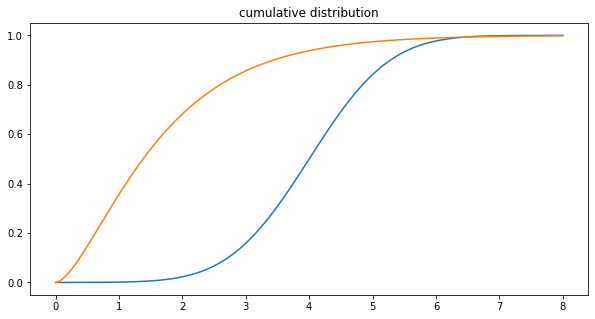
When the observed variable is continous (for example time), we speak of probability density function (PDF).In that case it does not give the exact probability of the variable taking a specific value (which would be 0), but the relative likelihood of the variable being equal to the value. The PDF can be used to determine the probability of a variable falling in the range of two values by computing the integral between those values.We can also use the cumulative distribution function (CDF), which is the probablity that the variable will be less or equal than the value.Given \(f_X(x)\) the PDF, then the CDF is \(F_{X}(x)=\int _{-\infty }^{x}f_{X}(t)\,dt.\)
- mode
The value that appears most often, that has the highest probability to happen. This can be seen as a peak (local maxima) of the PDF.
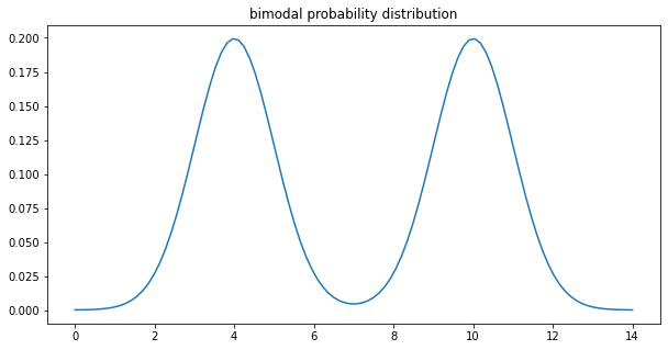
Most of the time there is only one such value, the distribution is then qualified as unimodal. But sometimes you will see bimodal distributions (or even multimodal ones).
If your benchmark has a bimodal distribution, then you probably want to rewrite it into two different benchmarks. This effectively means that your benchmark shows two distinct behaviors (probably code paths) with similar probability.

- skewness
Measures the asymmetry of the probability distribution of a random variable. For unimodal distributions, the skewness is
zero: if it is symmetric.
negative: if it has left tail (small values) is longer. The mass of the distribution is concentrated on the right of the figure.
positive: if it has a right tail (hihg values) is longer. The mass of the distribution is concentrated on the left of the figure.
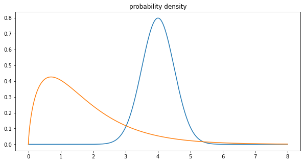
On the probability density function example image, the blue function is symmetric (zero skewness) while the orange function has positive skewness (right tail).
Note
In general, performance tests timings will have results with positive skewness.This can be explained easily: in ideal conditions, we would get a symmetrical distribution around the duration of the test.Most of the time values will be around the ideal case. But since a lot of random factors can slow the test, from time to time we get longer timings.Those factors do not always happen, but there are rare cases where it can accumulate and greatly be slowing down your test.Since there are (generally) more factors that can slow down the test than speed it up, you get a right tail longer than the left tail in the distribution. Hence the positive skewness.
Hypothesis testing
- population
- sample
- Population and samples are the base of statistical tests.In statistics, the population is a set of similar events or objects that are of interest with regard to an experiment. In terms of benchmarking, this is represents all the possible values your performance test can take.As one can not always collect all those results, we only use a subset of the population for our analysis, which is called the sample.
Note
For the sample to give a good representation of the whole population, elements must be chosen randomly and its size must be large enough.
- hypothesis testing
- This is a statistical test used to determine wether we can reject an hypothesis or not.The hypothesis we want to reject is called the null hypothesis (H0), and is paired with its opposite statement, the alternative hypothesis (H1).We call p-value the probability of H0 being true. Therefore we want it to be close to 0 to reject H0 and accept H1. In general, this is assumed once the p-value is inferior to a given significance level α (alpha).
- null hypothesis
- A statement used in hypothesis testing that denotes no relationship between multiple measurements. This is the statement we want to reject (prove that it is false).A p-value close to 0 means we can reject this hypothesis, if all other assumptions of the model are valid.
- alternative hypothesis
A statement in opposition to the null hypothesis. This is what we want to confirm. A p-value close to 0 means there are high chances that the alternative hypothesis is true, if all other assumptions of the model are valid.
- p-value
- probability value
- This is the best probability of obtaining test results as extreme as those in the observed sample.A very small p-value means that the observed outcome, while still possible, is not very likely under the null hypothesis. Which means our model (its assumptions and its null hypothesis) probably doesn’t fit the data.It is used to quantify the statistical significance of a test.
Warning
Statistical significance does not imply that the result is scientifically significant as well. This is just a tool to help you reach/invalidate conclusions, but it is not a proof.
In particular, all assumptions (shape of the data, how the experiment was conducted, …) other than the hypothesis must be valid so that we can deduce anything about the hypothesis using the p-value. [GSR16]
- significance level
- The probability of a test rejecting the null hypothesis, assuming it (and all the other assumptions of the model) to be true. If the p-value is inferior to the significance level, we then consider that the null hypothesis can be rejected.This is an arbitrary value chosen before the test, and is usually set to 5%, 1% or way lower depending on the required confidence.
References
- FW86
Fleming, P. & Wallace, J. (1986). How Not To Lie With Statistics: The Correct Way To Summarize Benchmark Results.. Commun. ACM. 29. 218-221. 10.1145/5666.5673.
- TEN15
Tene, G. (2015, September 28). How NOT to Measure Latency. Last accessed from https://www.youtube.com/watch?v=lJ8ydIuPFeU
- BAK19
Bakhvalov, D. (2019, December 30). Benchmarking: compare measurements and check which is faster. Last accessed from https://easyperf.net/blog/2019/12/30/Comparing-performance-measurements
- GSR16(1,2,3)
Greenland, S. & Senn, S.J. & Rothman, K.J. & al. (2016). Statistical tests, P values, confidence intervals, and power: a guide to misinterpretations. Eur J Epidemiol 31, 337–350. https://doi.org/10.1007/s10654-016-0149-3